⟨ψ| notes / quantum sensing
Double-quantum control and AC magnetometry in hBN
We use two synchronized microwave tones to control boron-vacancy spin ensembles in hexagonal boron nitride and measure an AC magnetic field.
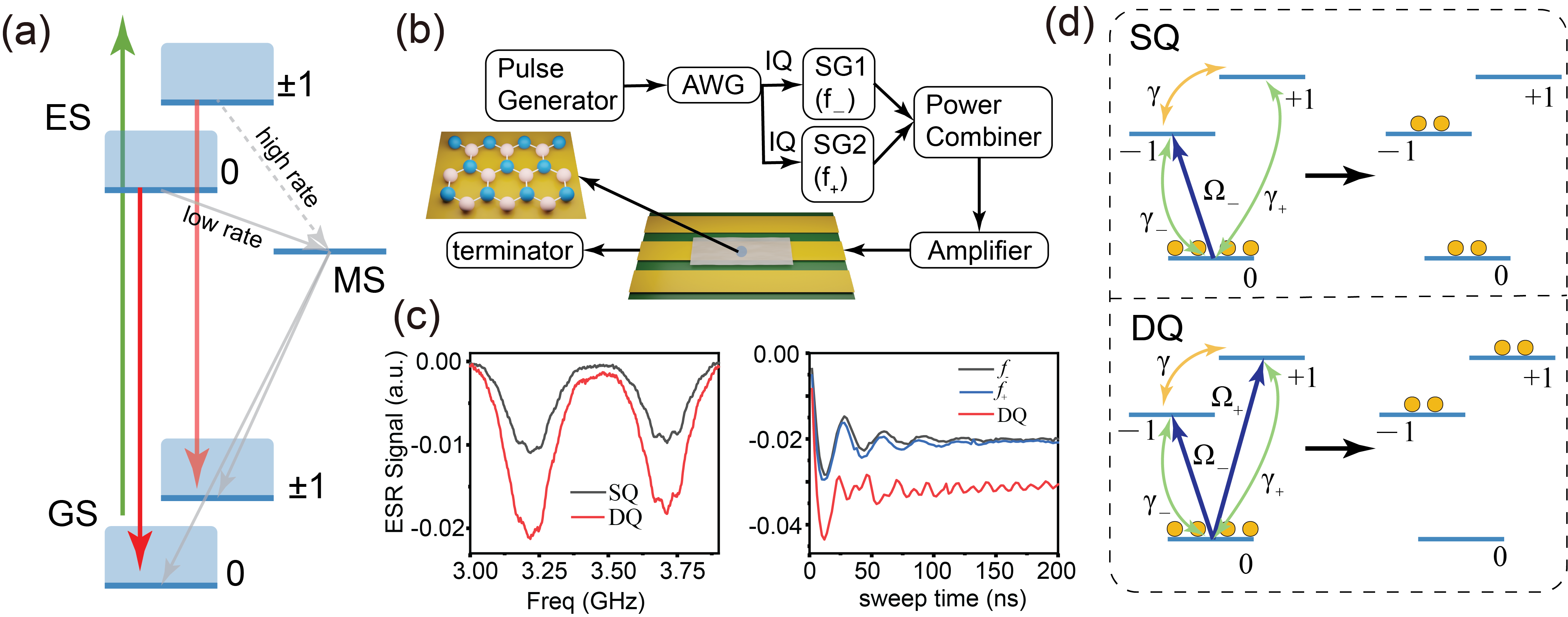
In the simple axial Zeeman picture, the two outer states of a spin triplet shift in opposite directions as the magnetic field changes. Their relative phase responds twice as strongly to the field as the phase between either outer state and |0⟩. This is the basis of double-quantum (DQ) sensing.
In our work accepted in Physical Review Applied, we use this coherence in negatively charged boron vacancies, VB−, in hBN. We detected an applied 20 MHz magnetic field and measured a 2.57-fold improvement in signal-to-noise ratio over single-quantum (SQ) control under the same experimental conditions.
Choosing the two outer spin states
The VB− ground state has spin projections ms = 0, +1, and −1. An SQ measurement uses a superposition of |0⟩ and one of the outer states. DQ sensing uses |+1⟩ and |−1⟩, whose spin projections differ by two.
In a simple axial-field picture, the two transition frequencies from |0⟩ are
Here γe is the electron gyromagnetic ratio in Hz/T, and Deff includes shifts shared by the two outer levels. Taking the frequency difference cancels this common contribution and doubles the magnetic-field slope relative to either SQ transition. We use this approximation when transverse mixing is small compared with the axial Zeeman splitting.
Fang and colleagues used quantum beats in diamond NV centres to suppress temperature- and strain-induced shifts of the common splitting. The doubled magnetic response includes magnetic noise. DQ control can therefore improve dephasing times when common shifts dominate, but it need not help when magnetic fluctuations dominate. Bauch and colleagues examined this dependence in NV ensembles.
Making DQ coherence in hBN
Two synchronized microwave tones drive the allowed transitions |0⟩ ↔ |+1⟩ and |0⟩ ↔ |−1⟩. We set their amplitudes, phases, and pulse durations to prepare coherence between the outer states. After the sensing interval, we map the accumulated phase onto spin populations and read them out through spin-dependent fluorescence.
The instruments share a 10 MHz reference, and an arbitrary waveform generator controls the microwave IQ modulation. We combine the two tones and deliver them through a coplanar waveguide. Green laser pulses provide initialization and readout of the defect ensemble in an hBN flake at room temperature.
For the hBN ensemble, the control has to work across a broadened set of resonances. We measured about twice the optical readout contrast with DQ driving as with SQ driving. Earlier work by Mamin and colleagues used dual-frequency DQ control for multipulse magnetometry with near-surface NV centres in diamond.
From a spin echo to an AC-field spectrum
A spin echo refocuses a static frequency offset. For an AC field, we time the spin inversion to a change in the field's sign so that the phase contributions before and after the inversion add. The pulse timing selects the frequency we sense. For an ideal DQ echo, the magnetic phase is
The switching function y(t) changes sign under the refocusing operation. This expression assumes ideal pulses and neglects their finite duration.
In correlation spectroscopy, we compare two sensing intervals separated by a variable delay. By scanning that delay and Fourier-transforming the resulting oscillation, we extract the field frequency. Laraoui and colleagues used this approach to resolve nuclear-spin signals near an NV centre over correlation times longer than a single electron-spin coherence interval.
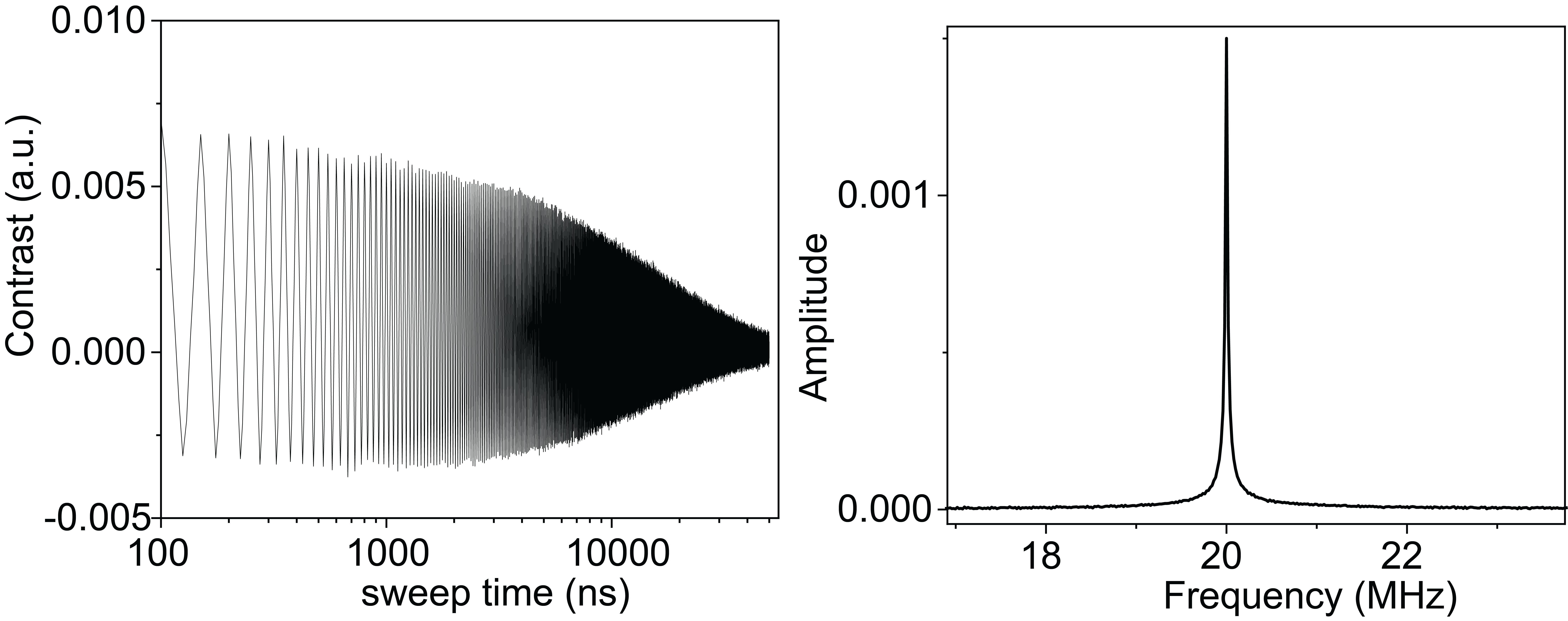
We applied a 20 MHz RF magnetic field with a nearby coil and found a peak at that frequency in the correlation spectrum. Without an applied RF signal, we observed a separate feature near 46.3 MHz, which we attribute to hyperfine coupling to nearby nuclear spins.
Reading the difference frequency with Qdyne
For quantum heterodyne detection, or Qdyne, we repeat the same sensing sequence at fixed intervals. Each fluorescence readout is timed against a stable classical clock. A difference between the field frequency and the timing reference produces a beat in this record.
The difference frequency is δ = fac − fref. In the small-signal regime, the phase-sensitive fluorescence follows the relative phase between the field and the sequence. Fourier-transforming the timed record gives the measured beat frequency.
Schmitt and colleagues and Boss and colleagues demonstrated frequency resolution far narrower than the inverse of a single spin-coherence time with clock-referenced readout. The spin can be reinitialized between measurements.
The sensing window sets how much phase we collect per block and which frequencies we detect. The repetition period sets the sampling rate and the resulting alias bands, while the total record length sets the Fourier-bin spacing. To assign an absolute frequency, we need the reference and the appropriate alias band. Clock stability and the coherence of the signal limit how far we can extend the useful record.
Rizzato and colleagues demonstrated RF sensing and coherently averaged synchronized readout (CASR) in hBN VB− ensembles. Here we use DQ coherence during the sensing interval and compare the readout with SQ control.
The measured signal-to-noise gain
We compare SQ and DQ control under the same Qdyne measurement conditions.
| Control | Signal-to-noise ratio |
|---|---|
| Single quantum | 100 |
| Double quantum | 257 |
| DQ / SQ | 2.57 |
The measured SNR depends on pulse fidelity, ensemble inhomogeneity, photon collection, and noise. We cannot predict it by multiplying the ideal phase-response gain by the optical contrast gain. The 2.57-fold result is the SNR ratio in this experiment. To quote an absolute sensitivity in T/√Hz, we would need a field calibration and a measurement-time normalization.
Improving control across the ensemble
To see where the DQ gain survives pulse errors, I would vary the microwave detuning and amplitude and measure both contrast and SNR. Hart and colleagues' DQ 4-Ramsey protocol uses phase cycling to reject residual SQ contributions in NV magnetic microscopy. Running the hBN measurement with and without phase cycling would test whether it reduces the residual SQ signal.
A calibrated RF field would let us compare the absolute sensitivities of the two protocols at equal acquisition times. Repeating the comparison for longer records would show how much further averaging improves each measurement.